Top 15 Advanced Excel Formulas Used in Data Operations – Syntax, Examples and Practical Uses

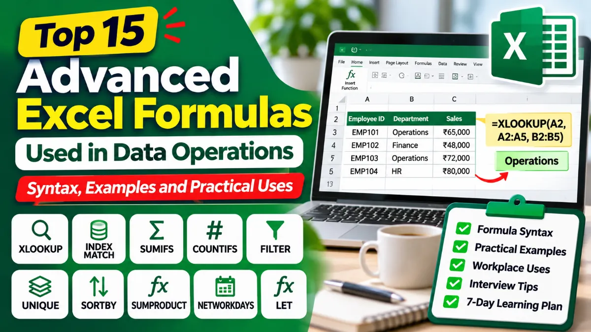
Basic Excel functions such as SUM, AVERAGE, and COUNT are useful for everyday calculations. However, data operations professionals often need advanced functions such as XLOOKUP, INDEX MATCH, SUMIFS, COUNTIFS, FILTER, IFERROR, SUMPRODUCT, and LET to handle more complicated tasks.

This article explains the top 15 advanced Excel formulas used in data operations, including their syntax, practical examples, common mistakes, and workplace applications. It also includes interview preparation tips and a seven-day learning plan for beginners.

Top 15 Advanced Excel Formulas – Quick Overview

The following table highlights important Excel functions and their practical applications.

Excel Formula	Primary Use	Common Application
XLOOKUP	Find matching records	Employee and customer databases
INDEX + MATCH	Flexible data lookup	Data reconciliation
SUMIFS	Calculate conditional totals	Sales and finance reports
COUNTIFS	Count matching records	Task and attendance tracking
IF + AND + OR	Apply decision rules	Eligibility and performance checks
IFERROR	Handle formula errors	Reporting and data validation
FILTER	Extract matching records	Pending task reports
UNIQUE	Identify distinct values	Customer and employee records
SORT + SORTBY	Arrange data dynamically	Performance rankings
SUMPRODUCT	Perform array calculations	Inventory valuation
TEXTJOIN	Combine text values	Employee and customer details
LEFT + RIGHT + MID	Extract text	Employee IDs and invoice numbers
TRIM + CLEAN	Clean imported data	Data processing
NETWORKDAYS	Calculate working days	HR and operations reporting
LET	Simplify complex formulas	Advanced MIS calculations

Excel compatibility: Some functions, including XLOOKUP, FILTER, UNIQUE, SORTBY, and LET, require Microsoft 365 or supported newer Excel versions, such as Excel 2024. They may not work in Excel 2016 or Excel 2019.

1. XLOOKUP – Find Matching Records Across Worksheets

XLOOKUP is one of the most useful Excel formulas for data operations. It searches for a value in one range and returns corresponding information from another range.

Data operations professionals use XLOOKUP to match employee IDs, customer numbers, invoice details, product codes, and transaction records.

XLOOKUP Formula Syntax

=XLOOKUP(lookup_value,lookup_array,return_array,[if_not_found])

Practical Example

Consider the following employee database.

Employee ID	Employee Name	Department
EMP101	Ravi	Finance
EMP102	Priya	HR
EMP103	Arun	Operations
EMP104	Sneha	IT

Suppose employee IDs are in A2, employee names in B2, and departments in C2.

To find the department of an employee whose ID is entered in E2, use:

=XLOOKUP(E2,A2:A5,C2:C5,”Not Found”)

If E2 contains EMP103, the result is Operations.

Real Workplace Application

An MIS executive receives an attendance report containing employee IDs but no department information. Instead of manually searching the employee database, XLOOKUP can retrieve department details automatically.

Important Tip: XLOOKUP performs exact matching by default. Check for extra spaces, inconsistent employee IDs, and incorrect data formats when records do not match.

2. INDEX + MATCH – Perform Flexible Data Lookups

The INDEX MATCH formula combines two Excel functions to retrieve information from a dataset.

INDEX returns a value from a specified position, while MATCH identifies the position of a matching record.

INDEX MATCH Formula Syntax

=INDEX(return_range,MATCH(lookup_value,lookup_range,0))

Practical Example

Using the employee database from the previous example:

=INDEX(B2:B5,MATCH(“EMP102”,A2:A5,0))

Result: Priya

MATCH identifies the position of EMP102 in the employee ID column. INDEX returns the corresponding employee name.

Real Workplace Application

INDEX MATCH is useful for employee record matching, inventory reconciliation, financial reporting, and maintaining older Excel workbooks.

XLOOKUP vs INDEX MATCH

Feature	XLOOKUP	INDEX MATCH
Ease of use	Generally easier	Requires combined functions
Exact matching	Default	Requires MATCH with 0
Lookup direction	Flexible	Flexible
Missing value handling	Built-in option	Usually combined with IFERROR
Older Excel compatibility	Limited	Better
Common use	Modern Excel reports	Legacy and specialized workbooks

Practical Recommendation: Learn XLOOKUP first if you use modern Excel. Learn INDEX MATCH as well because many organizations still maintain older spreadsheets.

3. SUMIFS – Calculate Totals Using Multiple Conditions

The SUMIFS formula calculates totals based on multiple conditions.

It is widely used in sales reporting, financial operations, branch-wise performance analysis, and monthly MIS reports.

SUMIFS Formula Syntax

=SUMIFS(sum_range,criteria_range1,criteria1,criteria_range2,criteria2)

Practical Example

Region	Department	Sales Amount
South	Electronics	₹45,000
North	Furniture	₹30,000
South	Electronics	₹25,000
South	Furniture	₹15,000
North	Electronics	₹20,000

To calculate total Electronics sales in the South region:

=SUMIFS(C2:C6,A2:A6,”South”,B2:B6,”Electronics”)

Result: ₹70,000

The formula adds ₹45,000 and ₹25,000 because both records satisfy the specified conditions.

Real Workplace Application

A sales operations executive can calculate revenue for a particular region, department, product category, or reporting period.

Common Mistake: The sum range and criteria ranges must have matching dimensions. Incorrect range selection can produce errors or misleading totals.

4. COUNTIFS – Count Records Using Multiple Conditions

COUNTIFS counts records that satisfy specified conditions.

This function is useful for tracking pending tasks, completed cases, employee attendance, customer complaints, and service performance.

COUNTIFS Formula Syntax

=COUNTIFS(criteria_range1,criteria1,criteria_range2,criteria2)

Practical Example

Employee	Department	Status
Ravi	Operations	Completed
Priya	HR	Pending
Arun	Operations	Pending
Sneha	Operations	Completed
Kiran	Operations	Pending

To count pending tasks assigned to the Operations department:

=COUNTIFS(B2:B6,”Operations”,C2:C6,”Pending”)

Result: 2

Real Workplace Application

A team leader can calculate the number of pending tasks for each department without manually filtering the entire dataset.

Practical Tip: Use cell references for criteria when creating dashboards. This makes reports easier to update.

5. IF + AND + OR – Apply Business Decision Rules

The IF function, combined with AND or OR, helps automate decisions based on business conditions.

These formulas are commonly used for employee incentives, attendance eligibility, quality checks, and performance classifications.

Practical Example – Employee Incentive Eligibility

Suppose employees qualify for an incentive when monthly sales are at least ₹50,000 and attendance is at least 90%.

=IF(AND(B2>=50000,C2>=90%),”Eligible”,”Not Eligible”)

Employee	Monthly Sales	Attendance	Result
Ravi	₹65,000	95%	Eligible
Priya	₹48,000	92%	Not Eligible
Arun	₹72,000	85%	Not Eligible

The formula returns Eligible only when both conditions are satisfied.

Using the OR Function

=IF(OR(B2>=50000,C2>=90%),”Review”,”Not Qualified”)

This formula returns Review when at least one condition is satisfied.

Also Read: Power BI Interview Questions and Answers Latest Update

Real Workplace Application

HR and operations teams use logical formulas to apply predefined business rules consistently across large datasets.

Important Difference: AND requires all conditions to be true, while OR requires at least one condition to be true.

6. IFERROR – Handle Missing Records and Formula Errors

Excel formulas may return errors such as #N/A, #DIV/0!, or #VALUE! when calculations fail or records cannot be found.

The IFERROR formula replaces an error result with a specified value or message.

IFERROR Formula Syntax

=IFERROR(value,value_if_error)

Practical Example

=IFERROR(B2/C2,0)

If C2 contains zero, the formula returns 0 instead of a division error.

Another example:

=IFERROR(INDEX(B2:B100,MATCH(E2,A2:A100,0)),”Not Found”)

If the employee ID is missing, Excel displays Not Found.

Real Workplace Application

Data operations professionals use IFERROR to make reports easier to read when some records are missing or calculations cannot be completed.

Important Tip: IFERROR does not correct the underlying data problem. In financial reports, displaying zero instead of an error can sometimes hide missing information. Use a message such as “Check Data” when further investigation is necessary.

7. FILTER – Extract Matching Records Automatically

The FILTER function extracts records that satisfy specified conditions.

Unlike manual filtering, FILTER produces a dynamic result that updates when the source data changes.

FILTER Formula Syntax

=FILTER(array,include,[if_empty])

Practical Example

Suppose A2 contains employee names, departments, and task statuses.

To display only pending records:

=FILTER(A2:C100,C2:C100=”Pending”,”No Records”)

The formula returns rows where the task status is Pending.

Real Workplace Application

A data operations executive can create a separate pending-task report that updates automatically when the source data changes.

Common Mistake: FILTER requires sufficient empty cells for its results. If the output area contains existing data, Excel may display a #SPILL! error.

8. UNIQUE – Identify Distinct Values in a Dataset

The UNIQUE function extracts distinct values from a selected range.

It is useful when working with customer lists, employee IDs, product categories, branch names, and transaction records.

UNIQUE Formula Syntax

=UNIQUE(array)

Practical Example

Customer ID
C101
C102
C101
C103
C102

Formula:

=UNIQUE(A2:A6)

Result: C101, C102, C103

To count distinct customer IDs:

=ROWS(UNIQUE(A2:A6))

Result: 3

Real Workplace Application

A customer operations team can identify the number of distinct customers appearing in a transaction dataset.

Identify Duplicate Records

To identify values that appear more than once:

=COUNTIF($A$2:$A$100,A2)>1

The formula returns TRUE when the value appears multiple times.

Important Tip: UNIQUE creates a separate distinct list. It does not remove records from the original dataset.

9. SORT + SORTBY – Organize Data Dynamically

The SORT and SORTBY functions arrange records without changing the original dataset.

SORT organizes a range using a selected column position, while SORTBY sorts records based on another range.

Practical Example

Suppose A2 contains employee names, departments, and monthly sales.

To sort the dataset by the third column in descending order:

=SORT(A2:C10,3,-1)

Alternatively:

=SORTBY(A2:C10,C2:C10,-1)

Both formulas arrange the records so that employees with the highest sales appear first.

Real Workplace Application

These formulas are useful for sales rankings, employee performance reports, inventory analysis, and task prioritization.

Important Tip: Always keep related columns together when sorting records. Sorting only employee names without their corresponding IDs or performance figures can damage data accuracy.

10. SUMPRODUCT – Calculate Weighted and Conditional Results

SUMPRODUCT multiplies corresponding values in arrays and adds the results.

It is useful for inventory valuation, financial calculations, weighted averages, and conditional reporting.

SUMPRODUCT Formula Syntax

=SUMPRODUCT(array1,array2)

Practical Example – Inventory Valuation

Product	Quantity	Unit Price
Keyboard	20	₹500
Mouse	30	₹300
Monitor	10	₹6,000

Formula:

=SUMPRODUCT(B2:B4,C2:C4)

Calculation:

• Keyboard: 20 × ₹500 = ₹10,000
• Mouse: 30 × ₹300 = ₹9,000
• Monitor: 10 × ₹6,000 = ₹60,000

Total Inventory Value: ₹79,000

Advanced Conditional Example

=SUMPRODUCT((A2:A100=”South”)*(B2:B100=”Completed”)*C2:C100)

This formula totals numeric values in column C for records where the region is South and the status is Completed.

Real Workplace Application

Inventory executives can calculate stock value without creating an additional column for each product’s total value.

Practical Recommendation: Use SUMIFS for straightforward conditional totals. SUMPRODUCT is especially useful when calculations involve multiple arrays.

11. TEXTJOIN – Combine Information From Multiple Cells

The TEXTJOIN formula combines text values using a specified separator.

It is commonly used for preparing employee details, customer information, addresses, and reporting labels.

TEXTJOIN Formula Syntax

=TEXTJOIN(delimiter,ignore_empty,text1,…)

Practical Example

First Name	Last Name	Department
Ravi	Kumar	Finance

Formula:

=TEXTJOIN(” – “,TRUE,A2:C2)

Result: Ravi – Kumar – Finance

Real Workplace Application

A data processing executive can combine employee details into standardized reporting fields.

Important Tip: Keep the original data columns when they are required for future filtering, validation, or analysis.

12. LEFT + RIGHT + MID – Extract Information From Text

Data operations teams frequently receive records containing employee codes, invoice IDs, transaction references, and product numbers.

The LEFT, RIGHT, and MID functions extract specific portions of text.

Practical Example

Suppose cell A2 contains:

EMP-2026-1045

Function	Formula	Result
LEFT	=LEFT(A2,3)	EMP
RIGHT	=RIGHT(A2,4)	1045
MID	=MID(A2,5,4)	2026

Real Workplace Application

These functions help extract department codes, year identifiers, invoice references, and product categories from standardized records.

Common Mistake: Fixed-position text extraction works best when all records follow the same format. If identifier lengths vary, TEXTBEFORE and TEXTAFTER may be more appropriate in supported Excel versions.

13. TRIM + CLEAN – Remove Unwanted Spaces and Characters

Poor data quality is a common problem in spreadsheet operations.

Employee names, customer IDs, and product descriptions may contain extra spaces or hidden characters introduced during copying or importing data.

TRIM removes leading and trailing ordinary spaces and reduces repeated spaces between words.

CLEAN removes certain nonprinting characters.

Practical Example

=TRIM(CLEAN(A2))

If A2 contains extra ordinary spaces around Ravi Kumar, the formula returns:

Ravi Kumar

Advanced Data Cleaning Formula

=TRIM(CLEAN(SUBSTITUTE(A2,CHAR(160),” “)))

This formula also handles nonbreaking spaces that may appear in copied web data.

Real Workplace Application

Data operations professionals can clean imported records before performing XLOOKUP, COUNTIFS, or reconciliation tasks.

Important Tip: Clean both datasets before matching records. Removing unwanted spaces from only one file may not solve every lookup problem.

14. NETWORKDAYS – Calculate Working Days Between Dates

The NETWORKDAYS function calculates the number of working days between two dates.

By default, it excludes Saturdays and Sundays. It can also exclude specified holidays.

NETWORKDAYS Formula Syntax

=NETWORKDAYS(start_date,end_date,[holidays])

Practical Example

If A2 contains the start date and B2 contains the completion date:

=NETWORKDAYS(A2,B2)

To exclude holidays listed in E2:E10:

=NETWORKDAYS(A2,B2,$E$2:$E$10)

Real Workplace Application

HR teams use this function for working-day calculations, while operations teams use it to measure turnaround times and service performance.

Important Tip: NETWORKDAYS includes both the start and end dates when they are working days. For organizations with different weekend schedules, NETWORKDAYS.INTL provides additional flexibility.

15. LET – Simplify Complex Excel Formulas

The LET function allows users to assign names to calculations within a formula.

This improves readability and reduces repeated calculations.

LET Formula Syntax

=LET(name1,value1,calculation)

Practical Example – Employee Performance Bonus

Suppose B2 contains monthly sales and C2 contains the sales target.

=LET(sales,B2,target,C2,IF(sales>=target,sales*5%,0))

If monthly sales are ₹80,000 and the target is ₹70,000, the result is:

₹4,000

Real Workplace Application

LET is useful for recurring performance calculations, complex MIS reports, financial models, and spreadsheets that require multiple calculations.

Practical Tip: Use meaningful variable names inside LET formulas so that other employees can understand and maintain the workbook.

Real Data Operations Example – Prepare an Employee Performance Report

Knowing individual Excel formulas is useful, but workplace assignments often require employees to combine multiple functions.

Consider the following sample task-processing report.

Employee ID	Department	Tasks Completed	Errors	Status
EMP101	Operations	120	2	Completed
EMP102	Finance	95	5	Pending
EMP103	Operations	150	1	Completed
EMP104	HR	80	4	Pending
EMP105	Operations	110	3	Completed

Assume the data is stored in A1.

Task 1 – Count Completed Records

=COUNTIF(E2:E6,”Completed”)

Result: 3

Task 2 – Calculate Tasks Completed by Operations Employees

=SUMIFS(C2:C6,B2:B6,”Operations”)

Result: 380

Task 3 – Find the Department of EMP103

=XLOOKUP(“EMP103″,A2:A6,B2:B6,”Not Found”)

Result: Operations

Task 4 – Calculate Total Errors

=SUM(D2:D6)

Result: 15

Task 5 – Calculate Overall Error Rate

=SUM(D2:D6)/SUM(C2:C6)

Result: Approximately 2.70%

Format the result cell as Percentage.

This calculation assumes that each error is counted against the reported number of completed tasks. Actual workplace quality metrics may use a different denominator.

Original Analysis – Why This Exercise Matters

A data operations report should answer more than one question.

Managers may need to know how many tasks were completed, which departments have pending work, whether error rates are increasing, and which records require investigation.

For example, the sample dataset shows that Operations employees completed 380 tasks, but the report alone does not explain whether that represents good performance. A meaningful evaluation also requires information about assigned workloads, targets, deadlines, and quality standards.

This is an important distinction between performing Excel calculations and interpreting operational data.

Advanced Excel Formulas for Different Job Roles

Different job positions require different combinations of Excel skills.

Job Role	Important Excel Formulas
Data Operations Associate	XLOOKUP, IFERROR, TRIM, COUNTIFS
MIS Executive	SUMIFS, COUNTIFS, FILTER, SORTBY
Data Analyst	FILTER, UNIQUE, SUMPRODUCT, LET
HR Operations Executive	XLOOKUP, IF, NETWORKDAYS
Finance Operations Associate	SUMIFS, INDEX MATCH, SUMPRODUCT
Back Office Executive	TEXTJOIN, LEFT, RIGHT, IFERROR
Inventory Executive	XLOOKUP, SUMPRODUCT, COUNTIFS

These are practical skill recommendations. Actual job requirements depend on the employer and position.

Important Excel Skills Beyond Formulas

Learning advanced formulas is only one part of becoming proficient in Excel.

Candidates preparing for data operations jobs, MIS executive positions, and Excel-based interviews should also understand the following features.

Also Read: LRS Services Hyderabad Data Entry Opeator Recruitment 2026 :Eiligibility and Full Details

Excel Skill	Workplace Importance
PivotTables	Summarize large datasets
Power Query	Import and transform recurring data
Conditional Formatting	Highlight errors and exceptions
Data Validation	Reduce incorrect data entry
Excel Tables	Maintain structured datasets
Charts and Dashboards	Present business performance
Data Reconciliation	Compare records across files
Power Pivot	Work with data models and relationships

For repeated monthly reporting tasks, Power Query may be more efficient than maintaining hundreds of formulas manually.

Common Excel Mistakes in Data Operations

Incorrect formulas are not the only reason reports fail. Data quality problems can also produce misleading results.

Common Mistake	Recommended Solution
Employee IDs do not match	Check spaces, formats, and leading zeros
Formula displays #N/A	Verify lookup values and ranges
Formula displays #SPILL!	Clear obstructing cells
Incorrect totals	Check conditions and selected ranges
Dates appear as text	Convert values into valid Excel dates
Formula references change when copied	Use absolute references such as $A$2
Duplicate records affect reports	Validate unique identifiers
IFERROR hides missing information	Investigate underlying errors
Numbers are stored as text	Convert values to numeric format
Source records are outdated	Verify data freshness before reporting

Practical Insight – A Correct Formula Can Still Produce a Wrong Report

Consider an employee database containing the same employee ID twice.

An XLOOKUP formula may return the first matching record correctly. However, if the first record contains outdated department information, the final report may still be wrong.

The formula is functioning as designed, but the underlying dataset requires validation.

Before preparing important reports, data operations professionals should check for duplicate identifiers, missing records, inconsistent formats, and outdated information.

Advanced Excel Interview Questions and Answers

1. Which Excel formula is best for matching employee IDs?

XLOOKUP is generally a convenient option in modern Excel because it supports exact matching, flexible return columns, and custom messages for missing records. INDEX MATCH is also useful, especially in older workbooks.

2. What is the difference between SUMIF and SUMIFS?

SUMIF calculates totals based on one condition, while SUMIFS supports multiple conditions.

For example, SUMIFS can calculate sales for a particular region and department simultaneously.

3. How can duplicate records be identified in Excel?

COUNTIF can identify repeated values, while Conditional Formatting can highlight duplicates. UNIQUE can generate a separate list of distinct values.

4. Which Excel formulas are useful for MIS reporting?

SUMIFS, COUNTIFS, XLOOKUP, FILTER, SORTBY, and IFERROR are particularly useful for preparing recurring MIS reports.

5. How do you clean imported Excel data?

TRIM, CLEAN, SUBSTITUTE, and suitable text-conversion functions can standardize imported records. Power Query is often better for recurring or large-scale data cleaning.

6. What is the difference between VLOOKUP and XLOOKUP?

VLOOKUP searches the first column of a selected table and returns a value using a column index.

XLOOKUP uses separate lookup and return ranges, making it more flexible and easier to maintain in many situations.

7. Is advanced Excel enough to get a data analyst job?

Advanced Excel provides a useful foundation, but many data analyst positions also require SQL, Power BI, statistics, or other analytical skills.

8. Which Excel formula should freshers learn first?

Freshers can begin with IF, COUNTIF, SUMIF, and basic lookups before moving to XLOOKUP, SUMIFS, COUNTIFS, FILTER, and SUMPRODUCT.

7-Day Advanced Excel Learning Plan

Candidates preparing for Excel-based jobs can follow this practical learning schedule.

Day	Topics	Practice Task
Day 1	XLOOKUP, INDEX MATCH	Match employee records
Day 2	SUMIFS, COUNTIFS	Prepare department-wise reports
Day 3	IF, AND, OR, IFERROR	Build performance rules
Day 4	FILTER, UNIQUE, SORTBY	Create a dynamic report
Day 5	TEXTJOIN, LEFT, RIGHT, MID, TRIM, CLEAN	Clean customer records
Day 6	SUMPRODUCT, NETWORKDAYS, LET	Calculate inventory and turnaround time
Day 7	Revision and mini-project	Prepare an operations MIS dashboard

Recommended Mini-Project

Create an employee performance workbook containing:

• Employee ID and department information
• Daily task completion records
• Error counts and pending cases
• Department-wise totals
• Employee performance rankings
• A separate report showing pending records
• Basic data-quality checks

Use XLOOKUP to retrieve employee information, SUMIFS for totals, COUNTIFS for pending cases, and FILTER to create a separate report.

A completed mini-project can provide practical evidence of Excel skills during job interviews.

Excel Skills for Freshers – What to Learn First

Fresh graduates do not need to master every advanced Excel function immediately.

A more practical learning order is:

Beginner Level: SUM, AVERAGE, COUNT, IF, COUNTIF, and basic data formatting.

Intermediate Level: XLOOKUP, INDEX MATCH, SUMIFS, COUNTIFS, IFERROR, and conditional formatting.

Advanced Level: FILTER, UNIQUE, SORTBY, SUMPRODUCT, LET, Power Query, and dashboard preparation.

Candidates applying for data operations positions should focus on accuracy, data cleaning, reporting, and problem-solving rather than memorizing formula names alone.

Official Microsoft Excel Learning Resources

Microsoft provides official documentation explaining Excel functions, syntax, and supported versions.

Resource	Official Website
Microsoft Excel Help	Check Now
XLOOKUP Function	Microsoft Xlookup Function
FILTER Function	Check Now
Excel Training and Support	https://support.microsoft.com/en-us/excel

Candidates should check the documentation for compatibility and additional examples when using different Excel versions.

Conclusion

Learning the top 15 advanced Excel formulas used in data operations can improve the accuracy, speed, and consistency of everyday reporting tasks.

For beginners, XLOOKUP, SUMIFS, COUNTIFS, IFERROR, and TRIM are particularly useful starting points because they address common workplace problems involving record matching, conditional calculations, task tracking, and data cleaning.

After gaining confidence with these functions, candidates can learn FILTER, UNIQUE, SORTBY, SUMPRODUCT, and LET to prepare more flexible reports.

However, Excel proficiency is not measured by the number of formulas someone remembers. Employers also value the ability to verify information, identify errors, explain results, and prepare reports that others can understand.

The best way to improve is to practise with realistic datasets, check the results carefully, and build small reporting projects that demonstrate practical problem-solving skills.